Instructions for the Revised 5-fund Spreadsheet

When you first open the file it may say it is a “Read Only” file; however, when you save the file on your hard drive you will be able to make changes and work in the spreadsheet. In the newer Excel version, you will need to click "Enable Content" in the yellow box at the top of worksheet.

After you have renamed the file and saved it to your hard drive (make sure you save in a location you can find it easily later such as your desktop).…close it and then reopen it.

Look at the bottom tabs.

The first tab is named Intro and contains information about the workbook and some tips for working in it.

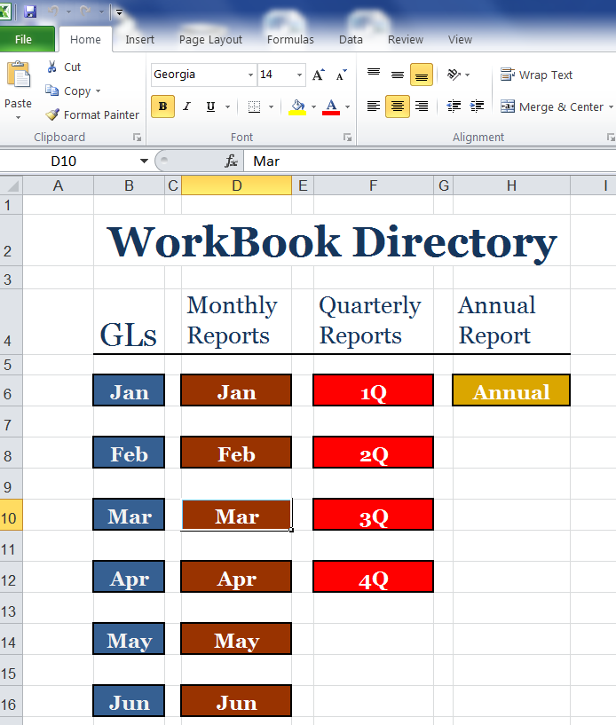
The second tab is the Directory worksheet. From this worksheet you can instantly go to any of the monthly, quarterly, and annual reports and any of the monthly general ledgers.

The third tab is your all-important Chart of Accounts. 

Here is where you will set up most of your information:

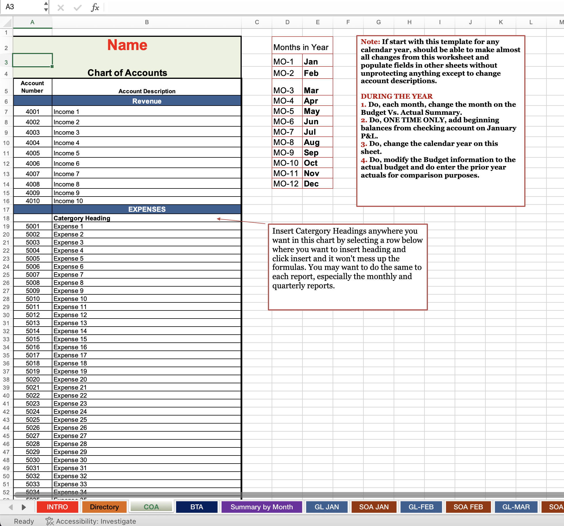
First step: Click in the heading and type in your organization’s name. (Notice that it auto filled into every worksheet (spreadsheet) from this one spreadsheet.)

This workbook (a single file containing a set of spreadsheets) is set up for 5 funds, 4 income accounts, and 40 expenses accounts. If you do not need that many funds or income and expenses accounts….don’t worry it is very easy to customize this workbook...if you need LESS of any those accounts.

So if you haven’t done it already, you need to figure out exactly how many funds you need to set up and how many income and expense accounts.

Take out a piece of paper and get to figuring:-) Please take a moment and read this page on fund accounting to refresh your memory on exactly what a fund is.

See tips on creating an effective chart of accounts!

After you have completed your chart of accounts…it’s time to start entering them into your accounting workbook.

Let’s set up your funds first. Scroll to the bottom of the worksheet (rows 61 to 65)

I have entered some funds for examples. Rename them.

If you do not need all 5 funds, it is very easy to hide what you do not need:

Go to the 6th tab (GL-Jan).

Highlight all the columns (Funds) you do not need; right click; go down to hide; and click. For example, say you only need 4 funds for right now. Highlight the columns P, Q and R…keeping your mouse positioned over the highlighted headings P, Q and R…right click….move down to HIDE and left click. You’ll notice your column headings now read …M, N, O, S, T…. The extra fund account is there hidden and can be “unhide” when you need another fund.

You will need to “hide” those extra fund columns on every worksheet in the workbook…except for the third worksheet. The tab is purple and titled “Summary by Month”. This sheet works only with the total columns. HOWEVER, you will need to hide any unwanted income or expense accounts on this worksheet. 

IMPORTANT-Hide the same columns and/or rows through the entire workbook.

For example: if you are hiding the 5th fund then make sure you hide the 5th fund throughout the workbook.

Next step: Enter the rest of your accounts. Notice that it auto filled into every worksheet (spreadsheet) from this one spreadsheet. This will make it much easier to make changes when needed.

Just like the funds it is easy to hide the income and expense accounts you don't need.

Go back to the 6th tab (GL-Jan).

Simply highlight all the rows you do not need; right click; go down to hide; and click. 

To "unhide" simply highlight the hidden rows --right click--left click on "unhide".

You will need to “hide” those extra income/expense accounts on every worksheet in the workbook.

IMPORTANT-Hide the same rows through the entire workbook.

If you need more funds or income/expenses accounts, see these pages for instructions on adding funds and income/expenses accounts.

However, unless you are very familiar with Excel or your spreadsheet program, I would strongly suggest using an accounting system such as Aplos Software as the spreadsheets are full of formulas and can be time consuming to add more accounts to.

After this is completed, save your workbook as original template and close it.

(Make sure you click YES if a pop up appears asking if you want to save your work:-)

Now open it again and save another copy for this year.

Entering Data:

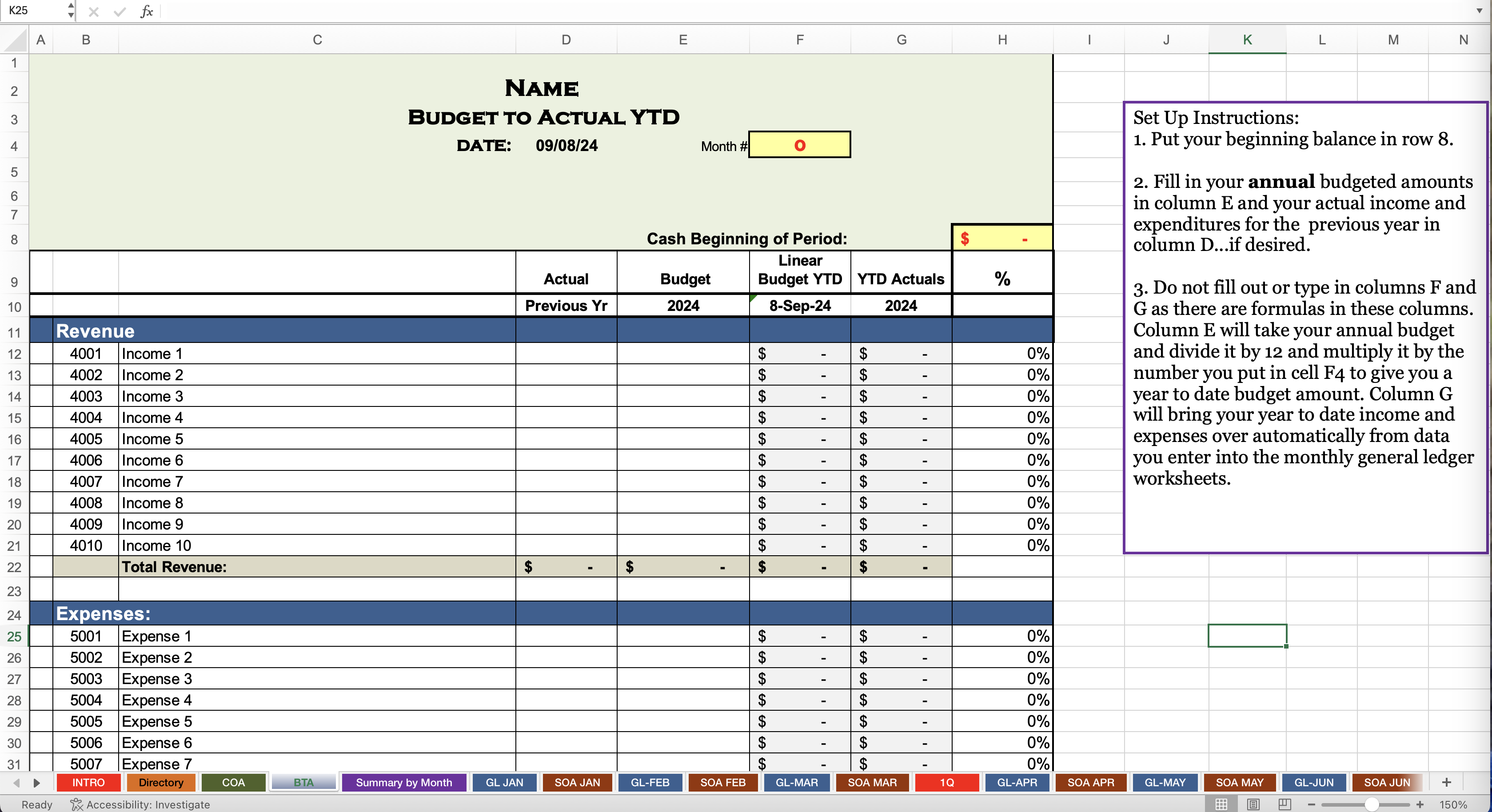
Go to the 4th worksheet (Tab titled BTA)

1. Put your beginning cash balance in first.

Fill in your annual budget  in column E and your actual income and expenditures for the previous year in column D...if desired.

Do not fill out or type in column F as there are formulas in this column to will take your annual budget and divide it by 12 and multiply it by the number you put in cell F4 to give you a year to date budget amount.

Do not fill out or type in column G as there are formulas in this column to bring your year to date income and expenses over automatically from the monthly general ledger reports.

You do not need to do anything to the next worksheet (Summary by Month). It will automatically fill in as you enter your expenses and income in the general ledgers.

Click on the 6th tab named GL-Jan. (There is a general ledger worksheet set up for each month) Each of these worksheets is where you will enter the data that the rest of the worksheets use to generate reports

• Contributions, fundraiser funds, etc. will be entered under its corresponding account in the credit (Income)column
• Utilities, office supplies, payroll, etc, will be entered under its corresponding account in the debit (Expense)column.
• Don’t worry if you accidentally delete a formula. Just click the “Go Back Button”.

Notice every time you enter an amount in a general ledger it is automatically carried to the monthly, quarterly, and annual reports; the Budget vs Actual report; and the Summary by Month report.

Note: If you add extra lines in your income/expense accounts, you will need to reset the balance column (see instructions for resetting it ).